Isotropic case for mouse brain did not yield any answers, although some tumours grew better especially when the number of time steps was increased. Tumours still stopped growing and concentration dropped to zero or negative.The upper video is of one of the best tumours, will run with same parameters to see if it can become any bigger.

A good example of an instability.   Will check data around this time that instability appears.

Mouse model instabilities 25/08/15

Progress: Simulations with conservative parameters of delta t have still been yielding unstable results.

As proliferation parameter rho is slowed down, the tumours look more real on the visualisation tools, to an extent.  They never grow to fill the whole brain, the ones that look solid even have an instability where they start shrinking and the concentration drops to zero, which implies an unstable data point somewhere in the tensor(?)

e.g.

The simulations are taking now 40+ minutes to run on my desktop PC and are becoming unrunnable apart from for time scales longer than about 23 days on my MacBook.

Data files are very large now due to the higher resolution so until I get stable solutions, I am just saving a record of the parameters I have varied with notes on how the solution behaved. 

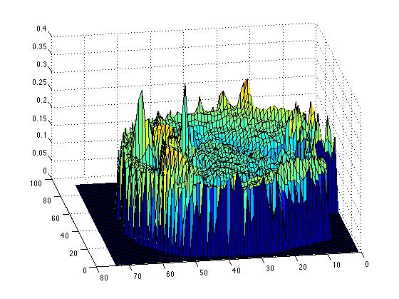
Looking at the diffusion tensor variable Mean_Diff, surface plot of slice (:,:,101), I will try running simulations at around (40,40,101) which will be away from the two spikes, although they are only a factor of two or so larger than the surrounding points.

Mouse Brain Simulations part 1:

After meetings at CAI and separately with Nyoman I have been working on processing the mouse brain data to simulate some tumours.  Initial results were flawed, after  a second attempt, where I understood the orientation and data better, I have produced a first simulation.

The anisotropy and diffusion are very apparent in this, presumably due to the much higher resolution images and more defined tracts.

Next step will be to compare this to tractography and make some slices, also repeat the process with the other mouse brain data Nyoman gave me.

A 7T Human image would be fantastic next.

EDIT:  I realised that the max tumour cell concentration was completely wrong as the human value had been used and the voxel size is 11680 times smaller in the mouse scan!

Hence the max tumour cell conc/voxel is around 20 in the mice scan using the same parameters.  Running this data now.

Centre for Advanced Imaging meeting and Mouse Brain Data

1. Following a meeting at CAI on Monday 03/08/2015, they have agreed to work with us and scan some of Simon Puttick's immunodeficient glioblastoma mice for us, to obtain a longitudinal data series. 
2. Nyoman Kurniawan, the small animal imaging expert at CAI has shared a 9.44T mouse brain atlas with us, which I have been working to put into the code and simulate tumours. I have done some of the preliminary processing, extracted the diffusion tensor, now to put in the new scan dimensions into our code.  The mouse brain has much smaller voxels and  is a different shape, the dimensions of the scan are 72x90x170, with the long axis inferior-superior (z-axis) because the mice are scanned vertically with the nose pointing to the sky. The hard bit here is lining up all the data, looking at the way it is organised in mrinfo for example to extract the right coordinates and so on. 

Wrote the following code to calculate the gradient of an isosurface of tumour to give a quantitative measure of shape:


%% gradient of a slice of tumour
% if not already defined, make Tumour from cstore
% for i = 1:201
% Tumour(:,:,:,i) =cstore{i};
% end
% then take time point t
% Tumour(t) = Tumour(:,:,:,t)
t = 200;
Slice = Tumour(:,:,40,t); %slice at z = 40, t = 125

%Manually make isosurface matrix
%RR = isosurface(Tumour80,2e5); then we have sructure RR.V (1613x3 double)
%and RR.F
RR = zeros(102,102);
ISO = Slice >2e5;
RR = RR + ISO;
%calculate gradient
%%Anisotropy Measure using gradient integral
%A quantitative measure of tumour anisotropy,
%1/(2*pi*R)*Integraldxdy* absolute value of grad phi
%discretised version:
%Sigma(ijk) abs(grad c(r)) =
%sqrt((partialc/partialx)^2+(partialc/partialy)^2+(partialc/partialz))dV
%partialc/partialx = ((Ci+1,j,k - Ci-1,j,k)/2deltax)

%practice code

dx = 1;
for i = 1:99, j = 1:100;
    dcdxsq =(RR(i+1,j) - RR(i,j)).^2;
end
for i=1:100, j = 1:99;
    dcdysq=(RR(i,j+1) - RR(i,j)).^2;
end
GridSum = sqrt(sum(sum(dcdxsq)) + sum(sum(dcdysq)));
figure
imagesc(RR)

GG=gradient(RR);
Aniso2 = sqrt(sum(sum(GG.^2)))
str = sprintf('Tumour surface = %f',Aniso2);
title(str);
%ThreeD version

TSurf = Tumour(:,:,:,t); %tumour matrix, t = 130
TIso = TSurf >2e5;
TTT = zeros(102,102,62);
TIso = TIso + TTT;
figure
fv = isosurface(TSurf,2e5);
p1 = patch(fv,'FaceColor','red','EdgeColor','none');
view(3)
daspect([1,1,1])
axis([0 100 0 100 0 60])
camlight
camlight(-80,-10)
lighting gouraud
title('Triangle Normals')
IsoGradient = gradient(fv.vertices);
AbsGrad3 = sqrt(sum(sum(IsoGradient.^2)))
str = sprintf('Tumour isosurface with Anisotropy = %f', AbsGrad3);
title(str)
%total tumour cells inside isosurface
ZZ = find(TSurf>2e5);
ZZZ= sum(sum(sum(ZZ)));

stf = sprintf('total tumour cells inside isosurface = %f', ZZZ)
str
Aniso2
AbsGrad3

Using this, I tabulated and plotted the data from a range of anisotropies using this code
%graphing anisotropy\
AnisoData = ...
[  NaN,      0,       1,            10,       15,         30,          45,       60,    100; ...
   NaN,    NaN,     NaN,           NaN,      NaN,         NaN,        NaN,      NaN,    NaN; ...
    40,      0,       0,             0,        0,          0,           0,        0,      0; ...
    50,      0,       0,          50.8308,  50.8358,     50.8358,    50.8572,   50.8621,   50.8690; ...
    60,   531.8208, 273.9941,    272.4435,  274.2529,   274.2529,   272.1032,   272.1409,  272.5392; ...
    70,   978.4913, 498.2811,    511.0714,  511.8223,   511.8223,   514.6845,   515.4931,  521.0318; ...
    80, 1.3849e+03, 764.0871,    784.7974,  787.4831,   787.4831,   802.9823,   802.8959,  809.3151; ...
    90, 1.8490e+03, 1.0832e+03, 1.1284e+03, 1.1359e+03, 1.1359e+03, 1.1695e+03, 1.1801e+03, 1.1909e+03; ...
   100, 2.3453e+03, 1.4825e+03, 1.5795e+03, 1.5993e+03, 1.5993e+03, 1.6569e+03, 1.6642e+03,1.6791e+03; ...
   110, 2.9061e+03, 1.9680e+03, 2.1226e+03, 2.1498e+03, 2.1498e+03, 2.2122e+03, 2.2211e+03,2.2375e+03; ...
   120, 3.4490e+03, 2.4469e+03, 2.6406e+03, 2.6727e+03, 2.6727e+03, 2.7469e+03, 2.7582e+03, 2.7812e+03; ...
   130, 3.9770e+03, 2.9079e+03, 3.1535e+03, 3.2000e+03, 3.2000e+03, 3.2964e+03, 3.3147e+03, 3.3333e+03; ...
   140, 4.4230e+03, 3.3718e+03, 3.6241e+03, 3.6663e+03, 3.6663e+03, 3.7589e+03, 3.7653e+03, 3.7858e+03; ...
   150, 4.6209e+03, 3.8110e+03, 4.0923e+03, 4.1365e+03, 4.1365e+03, 4.2477e+03, 4.2624e+03, 4.2996e+03; ...
   160, 4.8136e+03, 4.2563e+03, 4.5334e+03, 4.5946e+03, 4.5946e+03, 4.6870e+03, 4.6991e+03, 4.7366e+03; ...
   170, 4.9855e+03, 4.6604e+03, 4.9125e+03, 4.9501e+03, 4.9501e+03, 5.0425e+03, 5.0592e+03, 5.0788e+03; ...
   180, 5.1144e+03, 5.0263e+03, 5.1811e+03, 5.2162e+03, 5.2162e+03, 5.2552e+03, 5.2698e+03, 5.2814e+03; ...
   190, 5.2438e+03, 5.2282e+03, 5.2929e+03, 5.2902e+03, 5.2902e+03, 5.2949e+03, 5.2953e+03, 5.3019e+03; ...
   200, 5.2867e+03, 5.2929e+03, 5.2865e+03, 5.2865e+03, 5.2865e+03, 5.2865e+03, 5.2865e+03, 5.2865e+03];
X = AnisoData(3:end,1)*13.82;
Y0 = AnisoData(3:end,2);
Y1 = AnisoData(3:end,3);
Y10 = AnisoData(3:end,4);
Y15 = AnisoData(3:end,5);
Y30 = AnisoData(3:end,6);
Y45 = AnisoData(3:end,7);
Y60 = AnisoData(3:end,8);
Y100 = AnisoData(3:end,9);
plot(X,Y0, X,Y1, X,Y10, X,Y15, X,Y30, X,Y45, X,Y60, X,Y100)
axis([0 3000 0 5.5e3])
legend('y = rf0','y = rf1','y = rf10','y = rf15','y = rf30','y = rf45','y = rf60','y = rf100')
title('Plot of gradient of isosurface for varying anisotropy')
xlabel('time of tumour growth (days)')
ylabel('Abs(grad(isosurface))')

and produced some preliminaty graphs, which show the data behaves as expected and this may be a good measure of anisotropy of tumour surface.

Tomorrow I will explore the sum of tumour cell concentration within an isosurface as the anisotropy is varied. 

Then on to modelling resection.

Meeting with Z yesterday, plan is to explore virtual surgery this year, talk about experiments with mouse models next year and fully get to grips with what we have here and get my skills up a bit before moving on to more realistic simulations involving tissue mechanics. 
As Zoltan said, my skills are probably not up to tackling this kind of problem just yet, so this sems like a very good plan to me.

Anisotropy and Tissue Modelling progress

In the last fortnight I have met with Dr Yonghui Li, who kindly processed the tractography of the diffusion scan we have been working with and gave me a tutorial on the problems involved in doing this task.  Namely, making sure orientation and registration are correct while switching formats to MRTrix friendly files and processing.

I attended a Centre for Advanced Imaging seminar and there met Drs Gary Cowin, Nyoman Kurniawan and Andrew Janke, who showed me around and suggested that we do the deformation of the tissue modelling in a software package called ANTS (Advanced Normalisation of TissueS), which I downloaded and have not managed to compile successfully yet.

Further meeting to follow on Zoltan's return, Gary is the coordinator for imaging research and was very accommodating.

'Anisotropy'

Really we should be referring to surface irregularity?  

Finally got some working code, used the MATLAB \gradient function to calculate the gradient though, then took an absolute value of this. 

Using logical indexing to create a manual isosurface, we can get a matrix of ones, then we could use a nearest neighbours counting approach which I will start work on tomorrow, it should be reasonably straight forward, the question on whether it will provide any greater information than using the built in function is not really clear though.  

I also wrote code to show a movie of the surface plot of tumour evolution in a slice, which shows the traveling wave behaviour nicely.  

Found some code already written to view slice planes of a volume in MATLAB vis3d, which is very handy to have too. 

%% movie of surface plot of tumour cell density evolution in a slice
% if not already defined, make Tumour from cstore
% for i = 1:201
% Tumour(:,:,:,i) =cstore{i};
% end
% then take time point t
% Tumour(t) = Tumour(:,:,:,t)

Slice = Tumour80(:,:,40); %slice at z = 40

%Manually make isosurface matrix
%isoMatrix = Slice > 2e5;
%imagesc(Slice)
%figure
%surf(Slice)
colormap bone
caxis ([0 2.4e5])
colorbar

%make movie of surf plot
writerObj = VideoWriter('surfPlotofSlice.avi');
open(writerObj);
hold off
figure
for kk = 50:120
    Slice = Tumour(:,:,40,kk);
     surf(Slice)
     axis ([0 100 0 100 0 2.5e5])
    pause(0.1)
        frame = getframe;
        writeVideo(writerObj,frame);
colormap gray
caxis ([0 2.4e5])
end
close(writerObj);

Progress:

Monday July 06:

Working on anisotropy measures and visualisation of data. 

The simulation runs well now, I need to collect a new lot of data sets with the new boundary that includes the falx, but these can be ran as needed.

Exploration of the isosurface function in MATLAB has been productive, and 3D visualisation techniques have been explored and movies rendered.  

Dr Yonghui Li has provided me with a data set of processed tractography and given me a tutorial on how to do this myself, although I have not yet done so, nor was I able to open the data on my immediate attempt this morning.  

Next steps will be to explore the tractographic data and imaging tools associated with this and to produce a real anisotropy quantitative measure. 

Anisotropy:

A 2D toy model using a random grid was easily able to be implemented, however I have not yet been able to extend this to the 3D isosurface data produced.  

Tasks:  

1. Get a quantitative measure for the anisotropy of an isosurface.
2. Get a measure for total cell concentration within a given isosurface.
3. Measure the volume of the isosurface to compare with the surface area as a measure of smoothness.