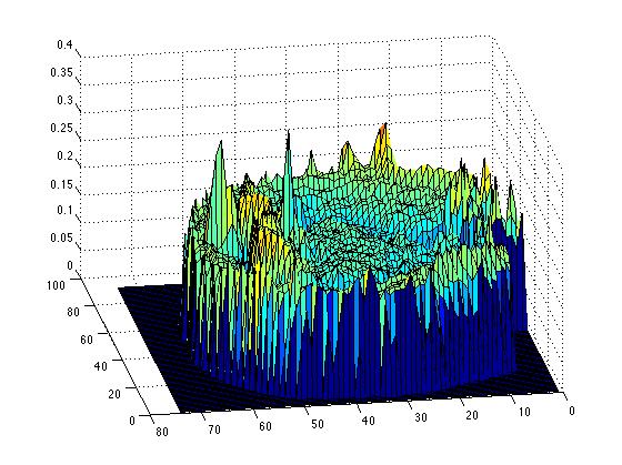
One dimensional surgery simulation has finally been successfully coded, taking out a segment and leaving that as space with a boundary as the simulation, we also tried stitching the function bak together, so there are two cases, in small tumours, the appropriate case would be stiching together, as the brain biomechanics would allow that degree of deformation, but in larger resections, the former case is more biologically appropriate.
Code:
%%1D-Fisher equation
%define constants
D = 2.5e-6; %Mean Cancer-cell Diffusion (mm^2/s)
rho = 4e-7; %Mean Cancer-cell growth rate (cells/second/voxel)
k = 2.4e5; %Maximum number of cells per unit volume (cells/mm^3)
%% Define Domain
%The size of DFull is 128*128*60*6. We choose n, m and p so that at full
%resolution (r=1) the size of D is 130*130*62*6, and we add a single layer
%of empty cells around the brain. This is just some insurance, because if
%the brain is touching the boundary of the domain, errors can occur.
%based on DTI data, 2.5mm voxels
%xpoints
xrange = [2.5:2.5:130*2.5]; %All these dimensions are in mm, and come straight from the MRI data
dx = 2.5; %space step size
xmax=max(xrange);
%right boundary
%m = floor(130); %ypoints
%p = floor(62); %zpoints
tsize =200; %tsteps. Unlike the space steps, this is variable. The stability condition requires it varies.
trange = [0, (2e8)]; %The time dimension in seconds
tmax=max(trange);
dt = (trange(2)-trange(1))/tsize; %time step size
tsteps = 1:dt:trange(2);
%stability
%% Initial Conditions
% Define Initial Condition as a function of x. Remember the units
% of c are cells per mm^3
% ic = @(x) 1*exp(-((x-mean(xrange))^2/1));
C=zeros(1,132); %initialise C
N = length(C);
C(62:67)=k/4; %I.C. cells here
CC = zeros(1,N); %post surgery function
%% Solve equation 1D FTCS scheme
%Explicitly step through time with anisotropic diffusion
%Equation dc/ct=D(\del^2)c + rho*c(1 -c/k), the Fisher KPP equation
%becomes in FTCS scheme
% c(i,k+1) = rc(i-1,k) + (1-2r)c(i,k) + rc(i+1,k)
% where r = Ddt/(dx)^2
%so set
r=((D*dt)/(dx)^2)
% Define C as a vector
%dCdt = (-2*D/dx^2).*C;
%C = C + dCdt*dt;
%C = C + dt*rho.*abs(C).*(1-abs(C)/k);
C(1) = 0;
C(132) = 0;
Cnew1 = zeros(1,N);
Cnew2 = zeros(1,N);
%C = C + dCdt*dt;
figure
hold off
ConcSumUncut=zeros(1,tsize);
for t=1:tsize
CC=C;
for i = 3:(N-2)
C(i) = r*CC(i+1) + (1-2*r)*CC(i) + r*CC(i-1);
end
%Also add a cell growth term - the Fisher Equation.
%Note the absolute values are just back-ups to ensure stability. We
%know that the explicit diffusion equation is numerically stable, as
%small disturbances will die down. But with an extra growth term, small
%disturbances may lead to negative numbers, which are then inflated.
%This is just a safety-measure.
C = C + dt*rho.*abs(C).*(1-abs(C)/k);
plot(CC) % ./k to normalise
axis([0 132 0 k])
pause(0.1)
disp(t)
%while t <= 30
%continue
% if t == 30 %then do surgery
%is=find(C>0.2*k,1)
%for i=1:N
% if C(i) < 0.2*k
%CC(i) = C(i);
% end
%end
%plot(N,CC)
%legend('Tumour', 'Resected tumour')
%for i = 1:(is-1)
Cnew1(i+((N/2)-is)+1) = CC(i);
%end
%for i = (N-is):N
Cnew2(i-(N/2-is)) = CC(i);
%end
%C = Cnew1 + Cnew2;
%feed this back into main loop
ConcSumUncut(t)=sum(C);
end
%plot(Csurg)
figure
plot(ConcSumUncut)
%end
%%Surgery function
%cuts C for C>is and stiches back together the ends
%%%One Dimensional tumour resection simulation. Boundary at cut edges.
%%post-resection.
%%1D-Fisher equation
%define constants
D = 2.5e-6; %Mean Cancer-cell Diffusion (mm^2/s)
rho = 4e-7; %Mean Cancer-cell growth rate (cells/second/voxel)
k = 2.4e5; %Maximum number of cells per unit volume (cells/mm^3)
%% Define Domain
%The size of DFull is 128*128*60*6. We choose n, m and p so that at full
%resolution (r=1) the size of D is 130*130*62*6, and we add a single layer
%of empty cells around the brain. This is just some insurance, because if
%the brain is touching the boundary of the domain, errors can occur.
%based on DTI data, 2.5mm voxels
%xpoints
xrange = [2.5:2.5:130*2.5]; %All these dimensions are in mm, and come straight from the MRI data
dx = 2.5; %space step size
xmax=max(xrange);
%right boundary
%m = floor(130); %ypoints
%p = floor(62); %zpoints
tsize =200; %tsteps. Unlike the space steps, this is variable. The stability condition requires it varies.
trange = [0, (2e8)]; %The time dimension in seconds
tmax=max(trange);
dt = (trange(2)-trange(1))/tsize; %time step size
tsteps = 1:dt:trange(2);
%stability
%% Initial Conditions
% Define Initial Condition as a function of x. Remember the units
% of c are cells per mm^3
% ic = @(x) 1*exp(-((x-mean(xrange))^2/1));
C=zeros(1,132); %initialise C
N = length(C);
C(62:67)=k/4; %I.C. cells here
CC = zeros(1,N); %post surgery function
%% Solve equation 1D FTCS scheme
%Explicitly step through time with anisotropic diffusion
%Equation dc/ct=D(\del^2)c + rho*c(1 -c/k), the Fisher KPP equation
%becomes in FTCS scheme
% c(i,k+1) = rc(i-1,k) + (1-2r)c(i,k) + rc(i+1,k)
% where r = Ddt/(dx)^2
%so set
r=((D*dt)/(dx)^2)
% Define C as a vector
%dCdt = (-2*D/dx^2).*C;
%C = C + dCdt*dt;
%C = C + dt*rho.*abs(C).*(1-abs(C)/k);
C(1) = 0;
C(132) = 0;
figure
hold off
ConcSum=zeros(1,tsize);
for t=1:30
CC=C;
for i = 2:(N-1)
C(i) = r*CC(i+1) + (1-2*r)*CC(i) + r*CC(i-1);
end
%Also add a cell growth term - the Fisher Equation.
%Note the absolute values are just back-ups to ensure stability. We
%know that the explicit diffusion equation is numerically stable, as
%small disturbances will die down. But with an extra growth term, small
%disturbances may lead to negative numbers, which are then inflated.
%This is just a safety-measure.
C = C + dt*rho.*abs(C).*(1-abs(C)/k);
% C = C + dt*0.001*rho.*abs(C).*(1-abs(C)/k).*(abs((C) - 0.2*k));
plot(CC) % ./k to normalise
axis([0 132 0 k])
pause(0.1)
disp(t)
%while t <= 30
%continue
if t == 30 %then do surgery
CC = zeros(1,N);
is=find(C>0.2*k,1);
for i=1:N
if C(i) < 0.2*k
CC(i) = C(i);
end
end
C = CC;
plot(CC)
%C(is+1) = C(is);
%C(N-is-1) = C(N-is);
%feed this back into main loop
end
ConcSum(t)=sum(C);
%plot(Csurg)
end
if i == is-1;
C(i) = (1-r)*CC(i) + r*CC(i-1);
if i ==(N-is+1);
C(i) = r*CC(i+1) + (1-r)*CC(i);
end
end
for t=31:tsize
CC=C;
for i=2:(is-2)
C(i) = r*CC(i+1) + (1-2*r)*CC(i) + r*CC(i-1);
end
for i=(N-is):N-1
C(i) = r*CC(i+1) + (1-2*r)*CC(i) + r*CC(i-1);
end
%for i = (N-is+1):(N-1)
% C(i) = r*CC(i+1) + (1-2*r)*CC(i) + r*CC(i-1);
%Also add a cell growth term - the Fisher Equation.
%Note the absolute values are just back-ups to ensure stability. We
%know that the explicit diffusion equation is numerically stable, as
%small disturbances will die down. But with an extra growth term, small
%disturbances may lead to negative numbers, which are then inflated.
%This is just a safety-measure.
C = C + dt*rho.*abs(C).*(1-(abs(C)/k));
%Cubic growth term?
%C = C + dt*0.001*rho.*abs(C).*(1-abs(C)/k).*abs((C-(0.02*k)./C));
plot(CC) % ./k to normalise
axis([0 132 0 (k)])
pause(0.1)
disp(t)
ConcSum(t) = sum(C);
end
figure
plot(ConcSum)
%end
%%Surgery function
%cuts C for C>is and stiches back together the ends
Code:
%%1D-Fisher equation
%define constants
D = 2.5e-6; %Mean Cancer-cell Diffusion (mm^2/s)
rho = 4e-7; %Mean Cancer-cell growth rate (cells/second/voxel)
k = 2.4e5; %Maximum number of cells per unit volume (cells/mm^3)
%% Define Domain
%The size of DFull is 128*128*60*6. We choose n, m and p so that at full
%resolution (r=1) the size of D is 130*130*62*6, and we add a single layer
%of empty cells around the brain. This is just some insurance, because if
%the brain is touching the boundary of the domain, errors can occur.
%based on DTI data, 2.5mm voxels
%xpoints
xrange = [2.5:2.5:130*2.5]; %All these dimensions are in mm, and come straight from the MRI data
dx = 2.5; %space step size
xmax=max(xrange);
%right boundary
%m = floor(130); %ypoints
%p = floor(62); %zpoints
tsize =200; %tsteps. Unlike the space steps, this is variable. The stability condition requires it varies.
trange = [0, (2e8)]; %The time dimension in seconds
tmax=max(trange);
dt = (trange(2)-trange(1))/tsize; %time step size
tsteps = 1:dt:trange(2);
%stability
%% Initial Conditions
% Define Initial Condition as a function of x. Remember the units
% of c are cells per mm^3
% ic = @(x) 1*exp(-((x-mean(xrange))^2/1));
C=zeros(1,132); %initialise C
N = length(C);
C(62:67)=k/4; %I.C. cells here
CC = zeros(1,N); %post surgery function
%% Solve equation 1D FTCS scheme
%Explicitly step through time with anisotropic diffusion
%Equation dc/ct=D(\del^2)c + rho*c(1 -c/k), the Fisher KPP equation
%becomes in FTCS scheme
% c(i,k+1) = rc(i-1,k) + (1-2r)c(i,k) + rc(i+1,k)
% where r = Ddt/(dx)^2
%so set
r=((D*dt)/(dx)^2)
% Define C as a vector
%dCdt = (-2*D/dx^2).*C;
%C = C + dCdt*dt;
%C = C + dt*rho.*abs(C).*(1-abs(C)/k);
C(1) = 0;
C(132) = 0;
Cnew1 = zeros(1,N);
Cnew2 = zeros(1,N);
%C = C + dCdt*dt;
figure
hold off
ConcSumUncut=zeros(1,tsize);
for t=1:tsize
CC=C;
for i = 3:(N-2)
C(i) = r*CC(i+1) + (1-2*r)*CC(i) + r*CC(i-1);
end
%Also add a cell growth term - the Fisher Equation.
%Note the absolute values are just back-ups to ensure stability. We
%know that the explicit diffusion equation is numerically stable, as
%small disturbances will die down. But with an extra growth term, small
%disturbances may lead to negative numbers, which are then inflated.
%This is just a safety-measure.
C = C + dt*rho.*abs(C).*(1-abs(C)/k);
plot(CC) % ./k to normalise
axis([0 132 0 k])
pause(0.1)
disp(t)
%while t <= 30
%continue
% if t == 30 %then do surgery
%is=find(C>0.2*k,1)
%for i=1:N
% if C(i) < 0.2*k
%CC(i) = C(i);
% end
%end
%plot(N,CC)
%legend('Tumour', 'Resected tumour')
%for i = 1:(is-1)
Cnew1(i+((N/2)-is)+1) = CC(i);
%end
%for i = (N-is):N
Cnew2(i-(N/2-is)) = CC(i);
%end
%C = Cnew1 + Cnew2;
%feed this back into main loop
ConcSumUncut(t)=sum(C);
end
%plot(Csurg)
figure
plot(ConcSumUncut)
%end
%%Surgery function
%cuts C for C>is and stiches back together the ends
%%%One Dimensional tumour resection simulation. Boundary at cut edges.
%%post-resection.
%%1D-Fisher equation
%define constants
D = 2.5e-6; %Mean Cancer-cell Diffusion (mm^2/s)
rho = 4e-7; %Mean Cancer-cell growth rate (cells/second/voxel)
k = 2.4e5; %Maximum number of cells per unit volume (cells/mm^3)
%% Define Domain
%The size of DFull is 128*128*60*6. We choose n, m and p so that at full
%resolution (r=1) the size of D is 130*130*62*6, and we add a single layer
%of empty cells around the brain. This is just some insurance, because if
%the brain is touching the boundary of the domain, errors can occur.
%based on DTI data, 2.5mm voxels
%xpoints
xrange = [2.5:2.5:130*2.5]; %All these dimensions are in mm, and come straight from the MRI data
dx = 2.5; %space step size
xmax=max(xrange);
%right boundary
%m = floor(130); %ypoints
%p = floor(62); %zpoints
tsize =200; %tsteps. Unlike the space steps, this is variable. The stability condition requires it varies.
trange = [0, (2e8)]; %The time dimension in seconds
tmax=max(trange);
dt = (trange(2)-trange(1))/tsize; %time step size
tsteps = 1:dt:trange(2);
%stability
%% Initial Conditions
% Define Initial Condition as a function of x. Remember the units
% of c are cells per mm^3
% ic = @(x) 1*exp(-((x-mean(xrange))^2/1));
C=zeros(1,132); %initialise C
N = length(C);
C(62:67)=k/4; %I.C. cells here
CC = zeros(1,N); %post surgery function
%% Solve equation 1D FTCS scheme
%Explicitly step through time with anisotropic diffusion
%Equation dc/ct=D(\del^2)c + rho*c(1 -c/k), the Fisher KPP equation
%becomes in FTCS scheme
% c(i,k+1) = rc(i-1,k) + (1-2r)c(i,k) + rc(i+1,k)
% where r = Ddt/(dx)^2
%so set
r=((D*dt)/(dx)^2)
% Define C as a vector
%dCdt = (-2*D/dx^2).*C;
%C = C + dCdt*dt;
%C = C + dt*rho.*abs(C).*(1-abs(C)/k);
C(1) = 0;
C(132) = 0;
figure
hold off
ConcSum=zeros(1,tsize);
for t=1:30
CC=C;
for i = 2:(N-1)
C(i) = r*CC(i+1) + (1-2*r)*CC(i) + r*CC(i-1);
end
%Also add a cell growth term - the Fisher Equation.
%Note the absolute values are just back-ups to ensure stability. We
%know that the explicit diffusion equation is numerically stable, as
%small disturbances will die down. But with an extra growth term, small
%disturbances may lead to negative numbers, which are then inflated.
%This is just a safety-measure.
C = C + dt*rho.*abs(C).*(1-abs(C)/k);
% C = C + dt*0.001*rho.*abs(C).*(1-abs(C)/k).*(abs((C) - 0.2*k));
plot(CC) % ./k to normalise
axis([0 132 0 k])
pause(0.1)
disp(t)
%while t <= 30
%continue
if t == 30 %then do surgery
CC = zeros(1,N);
is=find(C>0.2*k,1);
for i=1:N
if C(i) < 0.2*k
CC(i) = C(i);
end
end
C = CC;
plot(CC)
%C(is+1) = C(is);
%C(N-is-1) = C(N-is);
%feed this back into main loop
end
ConcSum(t)=sum(C);
%plot(Csurg)
end
if i == is-1;
C(i) = (1-r)*CC(i) + r*CC(i-1);
if i ==(N-is+1);
C(i) = r*CC(i+1) + (1-r)*CC(i);
end
end
for t=31:tsize
CC=C;
for i=2:(is-2)
C(i) = r*CC(i+1) + (1-2*r)*CC(i) + r*CC(i-1);
end
for i=(N-is):N-1
C(i) = r*CC(i+1) + (1-2*r)*CC(i) + r*CC(i-1);
end
%for i = (N-is+1):(N-1)
% C(i) = r*CC(i+1) + (1-2*r)*CC(i) + r*CC(i-1);
%Also add a cell growth term - the Fisher Equation.
%Note the absolute values are just back-ups to ensure stability. We
%know that the explicit diffusion equation is numerically stable, as
%small disturbances will die down. But with an extra growth term, small
%disturbances may lead to negative numbers, which are then inflated.
%This is just a safety-measure.
C = C + dt*rho.*abs(C).*(1-(abs(C)/k));
%Cubic growth term?
%C = C + dt*0.001*rho.*abs(C).*(1-abs(C)/k).*abs((C-(0.02*k)./C));
plot(CC) % ./k to normalise
axis([0 132 0 (k)])
pause(0.1)
disp(t)
ConcSum(t) = sum(C);
end
figure
plot(ConcSum)
%end
%%Surgery function
%cuts C for C>is and stiches back together the ends